HARISH POLA: ECE

clc;
clear all;
close all;
N=1024;
fs=8000;
f1=input('enter the 1st freuency');
f2=input('enter the 2nd freuency');
f3=input('enter the 3rd freuency');
n=0:N-1;
x=sin(2*pi*(f1/fs)*n)+sin(2*pi*(f2/fs)*n)+sin(2*pi*(f3/fs)*n);
figure(1)
pxx=spectrum(x,N)
specplot(pxx,fs);
grid ON;
xlabel('freq hz');
ylabel('mag in db');
title('power spectrum of x(n)');

Impulse Response of a First Order and Second Order System with Wave Forms

On 05:49 By hp // 1 comment:

clc;
clear all;
close all;
a=input('enter the numerator coefficient value');
b=input('enter the denominator coefficient value');
N=input('enter the number of samples');
[h,t]=impz(a,b,N);
disp('h=')
disp(h)
stem(t,h);
xlabel('samples');
ylabel('amplitude');
title('impulse response');

Dual Tone Multi Frequency with Waveforms

On 05:46 By hp // No comments:

clc;
clear all;
close all;
fs=8000;
f1=770+/fs;
f2=1209/fs;
n=1:205;
x1=sin(2*pi*f1*n);
x2=sin(2*pi*f2*n);
x=x1+x2;
y=fft(x,205);
K=1:50;
z(K)=y(K);
stem(K,abs(z));
xlabel('k');
ylabel('amplitude');
title('DTMF signal');

Implementation of Decimation / Interpolation Process with Waveforms

On 05:45 By hp // No comments:

clc;
clear all;
close all;
t=0:0.01:1;
d=input('enter number D/I');
x=sin(2*pi*5*t);
y=decimate(x,d);
subplot(3,1,1);
stem(x(1:25));
title('original input signal');
xlabel('samples');
ylabel('amplitude');
subplot(3,1,2);
stem(y);
title('decimated output');
xlabel('samples');
ylabel('amplitude');
y1=interp(y,d);
subplot(3,1,3);
stem(y1(1:25));
title('interpolation output');
xlabel('samples');
ylabel('amplitude');

Implementation of Decimation Process with Waveforms

On 05:43 By hp // No comments:

clc;
clear all;
close all;
x=input('enter the sequence');
d=input('enter the decimation factor');
N=length(x);
n=0:N-1;
xd=x(1:d:N);
n1=1:N/d;
subplot(2,1,1);
stem(n,x);
title('input signal');
xlabel('samples');
ylabel('amplitude');
subplot(2,1,2);
stem(n1-1,xd);
title('decimated output');
xlabel('samples');
ylabel('amplitude');

FFT and Convolution for FFT with Waveforms

On 05:42 By hp // No comments:

clc;
clear all;
close all;
x=input('enter the sequence');
N=input('enter the number of smples');
n=0:N-1
y=fft(x,N);
y1=abs(y);
y2=angle(y);
y3=ifft(y);
figure(1);
subplot(2,1,1);
stem(x);
title('original signal');
xlabel('samples');
ylabel('amplitude');
subplot(2,1,2);
stem(y);
title('fft signal');
xlabel('samples');
ylabel('amplitude');
figure(2);
subplot(2,1,1);
stem(y1);
title('magnitude plot');
xlabel('samples');
ylabel('amplitude');
subplot(2,1,2);
stem(y2);
title('phase angle');
xlabel('samples');
ylabel('amplitude');
figure(3);
subplot(2,1,1);
stem(y);
title('frequency domain sequence');
xlabel('samples');
ylabel('amplitude');
subplot(2,1,2);
stem(y3);
title('invers fft signal');
xlabel('samples');
ylabel('amplitude');

% CONV FOR FFT
clc;
clear all;
close all;
x=input('enter sequence of x');
h=input('enter sequence of h');
X1=[x zeros(1,length(h)-1)];
disp('X1=');
disp(X1);
h1=[h zeros(1,length(x)-1)];
disp('h1=');
disp(h1);
X=fft(x1);
H=fft(h1);
y=X.*H;
y1=ifft(y);
disp('the conv y1=');
disp(y1);
figure(1);
subplot(5,1,1);
stem(x);
title('input signal 1');
xlabel('samples');
ylabel('amplitude');
subplot(5,1,2);
stem(h);
title('input signal 2');
xlabel('samples');
ylabel('amplitude');
subplot(5,1,3);
stem(X1);
title('fft signal 1');
xlabel('samples');
ylabel('amplitude');
subplot(5,1,4);
stem(h1);
title('fft signal 2');
xlabel('samples');
ylabel('amplitude');
subplot(5,1,5);
stem(y1);
title('conv signal');
xlabel('samples');
ylabel('amplitude');

DFT and IDFT with Wave Forms

On 05:40 By hp // No comments:

clc;
clear all;
close all;
x=input('enter the input sequence');
L=length(x);
N=input('enter number of samples');
xn=[x zeros(1,N-L)]
n=[0:1:N-1]
k=[0:1:N-1]
wN=exp(-j*2*pi/N);
nk=n'*k;
wNnk=wN.^(nk);
xk=xn*wNnk;
disp('dft of given sequence');
disp(xk);
figure(1);
subplot(2,1,1);
stem(k,xn);
title('original samples');
xlabel('samples');
ylabel('amplitude');
subplot(2,1,2);
stem(k,xk);
title('discrete fourier transform');
xlabel('samples');
ylabel('amplitude');
figure(2)
subplot(2,1,1);
stem(k,abs(xk));
title('magnitude response');
xlabel('samples');
ylabel('amplitude');
subplot(2,1,2);
stem(k,angle(xk));
title('phase response');
xlabel('frequency');
ylabel('amplitude');

% IDFT
clc;
clear all;
close all;
x=input('enter the input sequence');
L=length(x);
N=input('enter number of samples');
xk=[x zeros(1,N-L)]
n=[0:1:N-1]
k=[0:1:N-1]
wN=exp(-j*2*pi/N);
nk=n'*k;
wNnk=wN.^(-nk);
xn=(xk*wNnk)/N;
disp('dft of given sequence');
disp(xk);
figure(1);
subplot(2,1,1);
stem(k,xk);
title('original samples');
xlabel('samples');
ylabel('amplitude');
subplot(2,1,2);
stem(k,xn);
title('discrete fourier transform');
xlabel('samples');
ylabel('amplitude');

Frequency Response of a Given System with Wave Forms

On 05:37 By hp // No comments:

%impulse response
clc;
clear all;
close all;
N=input('enter the length of the sequence');
a=input('enter the numerator coefficient value');
b=input('enter the denominator coefficient value');
n1=0:1:N-1;
x1=(n1==0);
h1=filter(b,a,x1);
disp(h1);
subplot(2,1,1);
stem(n1,x1);
title('impulse response');
xlabel('samples');
ylabel('amplitude');
subplot(2,1,2);
stem(n1,h1);
xlabel('samples');
ylabel('amplitude');

%unit step

clc;
clear all;
close all;
N=input('enter the length of the sequence');
a=input('enter the numerator coefficient value');
b=input('enter the denominator coefficient value');
n1=0:1:N-1;
x1=(n1>=0);
h1=filter(b,a,x1);
disp(h1);
subplot(2,1,1);
stem(n1,x1);
title('unit step response');
xlabel('samples');
ylabel('amplitude');
subplot(2,1,2);
stem(n1,h1);
xlabel('samples');
ylabel('amplitude');
% cosine signal
clc;
clear all;
close all;
N=input('enter the length of the sequence');
a=input('enter the numerator coefficient value');
b=input('enter the denominator coefficient value');
n1=0:1:N-1;
x1=cos(0.05*pi*n1);
h1=filter(b,a,x1);
disp(h1);
subplot(2,1,1);
stem(n1,x1);
title('cos signal');
xlabel('samples');
ylabel('amplitude');
subplot(2,1,2);
stem(n1,h1);
xlabel('samples');
ylabel('amplitude');

Generation of Elementary Sequences of All Signals with Wave Forms

On 05:27 By hp // No comments:

%impulse
clc;
clear all;
close all;
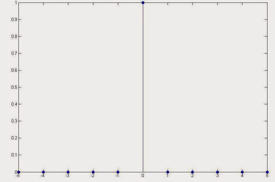
disp('unit impulse signal');
N=input('enter number of samples');
n=-N:1:N
X=(n==0)
stem(n,X,'filled');
x label('samples');
y label(amplitude');
title('impulse signal');
%unit step
clc;
clear all;
close all;
disp('unit step signal');
N=input('enter number of samples');
n=-N:1:N
X=(n>=0)
stem(n,X,'filled');
x label('samples');
y label(amplitude');
%unit ramp
clc;
clear all;
close all;
disp('unit ramp signal');
N=input('enter number of samples');
a=input('enter value of ramp');
n=0:0.5:N
X=a*n
stem(n,X,'filled');
x label('samples');
y label(amplitude');
%exponential
clc;
clear all;
close all;
disp('growing exponential signal');
N=input('enter number of samples');
a=input('enter value of a');
n=-N:1:N
X=a.^n
stem(n,X,'filled');
xlabel('samples');
ylabel('amplitude');
%sine signal
clc;
clear all;
close all;
disp('sine signal');
N=input('enter number of samples');
n=0:0.1:N
X=sin(n)
stem(n,X,'filled');
xlabel('samples');
ylabel('amplitude');
%cosine signal
clc;
clear all;
close all;
disp('cosine signal');
N=input('enter number of samples');
n=0:0.1:N
X=cos(n)
stem(n,X,'filled');
xlabel('samples');
ylabel('amplitude');

Ac Matlab Outputs

On 09:15 By hp // No comments:

JUST CLICK ON BELOW SITE THAT SHOWS A FILE NAMED acoutput11.10.2014.docx (219,2 kB) CLICK ON THAT DIRECT WORD FILE WILL DOWNLOAD U CAN GOTHROUGH THE OUTPUTS THERE .......

http://harishpola.webnode.com/news/ac-matlab-outputs/

Frequency Modulation Using Message Signal as A Square in Matlab with Waveforms

On 09:37 By hp // 2 comments:

clc;
clear all;
close all;
fc=30;
fm=2;
dev=20;
fs=100*fc;
t=0:1/fs:2/fm;
mt=square(2*pi*fm*t);
ct=sin(2*pi*fc*t);
st1=fmmod(mt,fc,fs,dev);
st2=pmmod(mt,fc,fs,dev);
figure(1);
subplot(4,1,1);
plot(t,mt,'r');
title('msg signal');
xlabel('time');
ylabel('amplitude');
subplot(4,1,2);
plot(t,ct);
title('carrier signal');
xlabel('time');
ylabel('amplitude');
subplot(4,1,3);
plot(t,st1);
title('fm modulated signal');
xlabel('time');
ylabel('amplitude');
subplot(4,1,4);
plot(t,st2);
title('pm modulated signal');
xlabel('time');
ylabel('amplitude');

Frequency Synthesizer Using Matlab with Waveforms

On 09:34 By hp // No comments:

clc;
clear all
close all;
fs=10000;
t=0:1/fs:1;
f=10;
x1=square(2*pi*f*t);
x2=square(2*pi*f/2*t);
x3=square(2*pi*2*f*t);
subplot(3,1,1);
plot(t,x1,'g');
title('original signal');
xlabel('time period');
ylabel('frequency');
subplot(3,1,2);
plot(t,x2,'r');
title('original signal with half frequency');
xlabel('time period');
ylabel('frequency');
subplot(3,1,3);
plot(t,x3,'b');
title('original signal with double frequency');
xlabel('time period');
ylabel('frequency');

Sampling Theorem Using Matlab with Waveforms

On 09:33 By hp // No comments:

clc;
clear all;
close all;
t=-10:0.01:10;
T=4;
fm=1/T;
x=cos(2*pi*fm*t);
subplot(2,2,1);
plot(t,x);
title('msg signal');
xlabel('time');
ylabel('amplitude');
fs1=1.6*fm;
fs2=2*fm;
fs3=8*fm;
%sampling with fs<2fm
n1=-4:1:4;
x1=cos(2*pi*fm/fs1*n1);
subplot(2,2,2);
stem(n1,x1);
hold on;
subplot(2,2,2);
plot(n1,x1,'r');
title('sampling when fs<2fm ');
xlabel('sample');
ylabel('amplitude');
%sampling with fs=2fm
n2=-5:1:5;
x2=cos(2*pi*fm/fs2*n2);
subplot(2,2,3);
stem(n2,x2);
hold on;
subplot(2,2,3);
plot(n2,x2,'r');
title('sampling when fs=2fm ');
xlabel('sample');
ylabel('amplitude');
%sampling with fs>2fm
n3=-20:1:20;
x3=cos(2*pi*fm/fs3*n3);
subplot(2,2,4);
stem(n3,x3);
hold on;
subplot(2,2,4);
plot(n3,x3,'r');
title('sampling when fs>2fm ');
xlabel('sample');
ylabel('amplitude');